Examples
These are examples for the bare afmformats package. You might find other examples interesting to you in the nanite documentation.
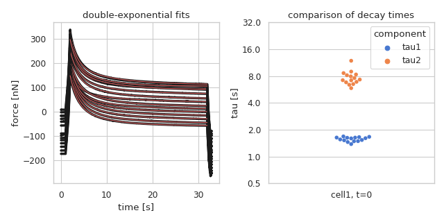
Double-exponential fit to stress-relaxation data
This example reproduces the first entry in figure 5d (cell1) of [BAZ+22].
Please note that in the original manuscript, not all curves were used in the final figure. Some curves were excluded based on curve quality. The data were kindly provided by Alice Battistella.
 1import pathlib
 2import shutil
 3import tempfile
 4
 5import afmformats
 6
 7from lmfit.models import ConstantModel, ExponentialModel
 8import matplotlib.pylab as plt
 9from matplotlib.ticker import ScalarFormatter
10import numpy as np
11import pandas
12import seaborn as sns
13sns.set_theme(style="whitegrid", palette="muted")
14
15
16# extract the data to a temporary directory
17data_path = pathlib.Path(__file__).parent / "data"
18wd_path = pathlib.Path(tempfile.mkdtemp())
19shutil.unpack_archive(data_path / "10.1002_btm2.10294_fig5d-cell1.zip",
20                      wd_path)
21
22# scale conversion constants
23xsc = 1
24ysc = 1e9
25xl = "time [s]"
26yl = "force [nN]"
27
28# data extraction
29data = []
30for path in wd_path.glob("*.jpk-force"):
31    data += afmformats.load_data(path)
32
33# this is where the data for the swarm plot is stored
34rdat = {
35    "tau": [],
36    "component": [],
37    "cell": [],
38}
39
40data_fits = []
41
42for di in data:
43    # use intermediate `intr` segment data
44    x = di.intr["time"] * xsc
45    y = di.intr["force"] * ysc
46
47    # fitting with double-exponential
48    const = ConstantModel()
49    exp_1 = ExponentialModel(prefix='exp1_')
50    exp_2 = ExponentialModel(prefix='exp2_')
51
52    pars = exp_1.guess(y, x=x)
53    pars.update(exp_2.guess(y, x=x))
54    pars["exp1_decay"].set(value=1, min=0.1)
55    pars["exp2_decay"].set(value=8, min=2)
56    pars.update(const.guess(y, x=x))
57    pars["c"].set(value=np.min(y))
58
59    mod = const + exp_1 + exp_2
60
61    init = mod.eval(pars, x=x)
62    out = mod.fit(y, pars, x=x)
63    data_fits.append([x, out.best_fit])
64
65    rdat["tau"].append(out.params["exp1_decay"].value)
66    rdat["component"].append("tau1")
67    rdat["cell"].append("cell1, t=0")
68
69    rdat["tau"].append(out.params["exp2_decay"].value)
70    rdat["component"].append("tau2")
71    rdat["cell"].append("cell1, t=0")
72
73
74fig = plt.figure(figsize=(8, 4))
75
76# plot all stress-relaxation curves
77ax1 = plt.subplot(121, title="double-exponential fits")
78for ii in range(len(data)):
79    di = data[ii]
80    ax1.plot(di["time"]*xsc, di["force"]*ysc, color="k", lw=3)
81    xf, yf = data_fits[ii]
82    ax1.plot(xf, yf, color="r", lw=1)
83ax1.set_xlabel(xl)
84ax1.set_ylabel(yl)
85
86df = pandas.DataFrame(data=rdat)
87# Draw a categorical scatterplot to show each observation
88ax2 = plt.subplot(122, title="comparison of decay times")
89ax2 = sns.swarmplot(data=df, x="cell", y="tau", hue="component")
90ax2.set_yscale('log', base=2)
91ax2.yaxis.set_major_formatter(ScalarFormatter())
92ax2.set_yticks([0.5, 1, 2, 4, 8, 16, 32])
93ax2.set(xlabel="", ylabel="tau [s]")
94
95plt.tight_layout()
96
97plt.show()